Combination

Since the order of the prisoners doesn’t matter, the problem is a combination question. In conventional combinations, the number of \(k\)-combinations of a \(n\)-element set (\(k \leq n\)) is equal to the binomial coefficient \({{n}\choose{k}} = \frac{n!}{k!(n-k)!} = \frac{n(n-1)...(n-k+1)}{k(k-1)...1}\). For example, there are \({{3}\choose{2}} = \frac{3 \times 2}{2 \times 1} = 3\) ways to choose a 2-element tuple from a 3-element set \(\{A, B, C\}\), namely \((A, B)\), \((A, C)\), and \((B, C)\).

Conventional combinations are drawn without repetition. The 3 tuples in the previous example are all unique sets. However, in our prisoner problem, the same prisoner can be taken more than once, so the binomial coefficient doesn’t seem to apply here.

What we need here is a way to count multisets. Formally, the number of multisets of cardinality \(k\), with elements taken from a finite set of cardinality \(n\), is the multiset coefficient, written as \(\left(\!\!{n\choose k}\!\!\right)\).

The value of multiset coefficient can be computed using an equivalent binomial coefficient.

\[\left(\!\!{n\choose k}\!\!\right) = {{n+k-1}\choose{k}} = \frac{(n+k-1)!}{k!(n-1)!}\]

To see this equivalence, one can use a simple technique called stars and bars.

Suppose 3 elements are drawn with repetition from the set \(\{1,2\}\) of cardinality 2 (\(n=2, k=3\)). It’s not difficult to enumerate all possible multisets because there are only 4 of them: \(\{1,1,1\}\), \(\{1,1,2\}\), \(\{1,2,2\}\), and \(\{2,2,2\}\).

We can also represent those multisets in another form.

\(\{{\bullet}{\bullet}{\bullet}|\}\), \(\{{\bullet}{\bullet}|{\bullet}\}\), \(\{{\bullet}|{\bullet}{\bullet}\}\), and \(\{|{\bullet}{\bullet}{\bullet}\}\)

In this form, all elements are denoted as a dot. Vertical bars are put to divide the dots into bins, with each bin representing an element from the unique set. It’s possible to have a bin with no elements which basically means that the particular unique element doesn’t have any corresponding elements in the multiset (e.g., the first multiset doesn’t have element \(2\) and the last multiset doesn’t have \(1\)).

One needs \(n-1\) bars to represent a unique set of cardinality \(n\). If we count the total number of dots and bars in a \(k\)-element multiset, it’s \(k+n-1\). Then the total number of possible \(k\)-element multisets equals to the total number of ways of placing \(n-1\) bars in \(k+n-1\) items, which is \({{k+n-1}\choose{n-1}} = {{k+n-1}\choose{k}}\).

The denominator

Let’s return to the original question. What’s the probability of all prisoners being taken to the room at least once after the warden takes \(k\) times? To compute this probability, We need to compute the total number of possible scenarios which will serve as the denominator.

The total number should equal to \(\left(\!\!{n\choose k}\!\!\right)\), for a \(k \geq n\). From the previous section, We can work out \(\left(\!\!{n\choose k}\!\!\right) = {{k+n-1}\choose{k}}\).

The numerator

The numerator of the probability is the number of multisets in which all prisoners are present at least once. The trick to compute this number is to divide any such multiset into two parts: one set that contains all 100 prisoners and the other with remaining \(k-100\) elements. Then the total number of such multisets equals to \(\left(\!\!{n\choose k-n}\!\!\right) = {{n+k-n-1}\choose{n-1}} = {{k-1}\choose{n-1}}\), for a \(k \geq n\).

The probability

Once we have both the denominator and numerator, the probability is straightforward to compute.

\[Pr(n,k) = \frac{{{k-1}\choose{n-1}}}{{{k+n-1}\choose{k}}} = \frac{\frac{(k-1)!}{(n-1)! \cdot (k-n)!}}{\frac{(k+n-1)!}{k! \cdot (n-1)!}} = \frac{k!(k-1)!}{(k+n-1)!(k-n)!}\]

In our case, \(n=100\), so

\[Pr(100,k) = \frac{k!(k-1)!}{(k+99)!(k-100)!}\]

We can plot this probability function for \(100 \leq k \leq 200\).

Pr <- function(k) {
  choose(k-1, 99)/choose(k+99, k)
}
ggplot() +
  xlim(100, 200) +
  geom_function(fun = Pr) +
  labs(x = "k", y = "Pr(100, k)")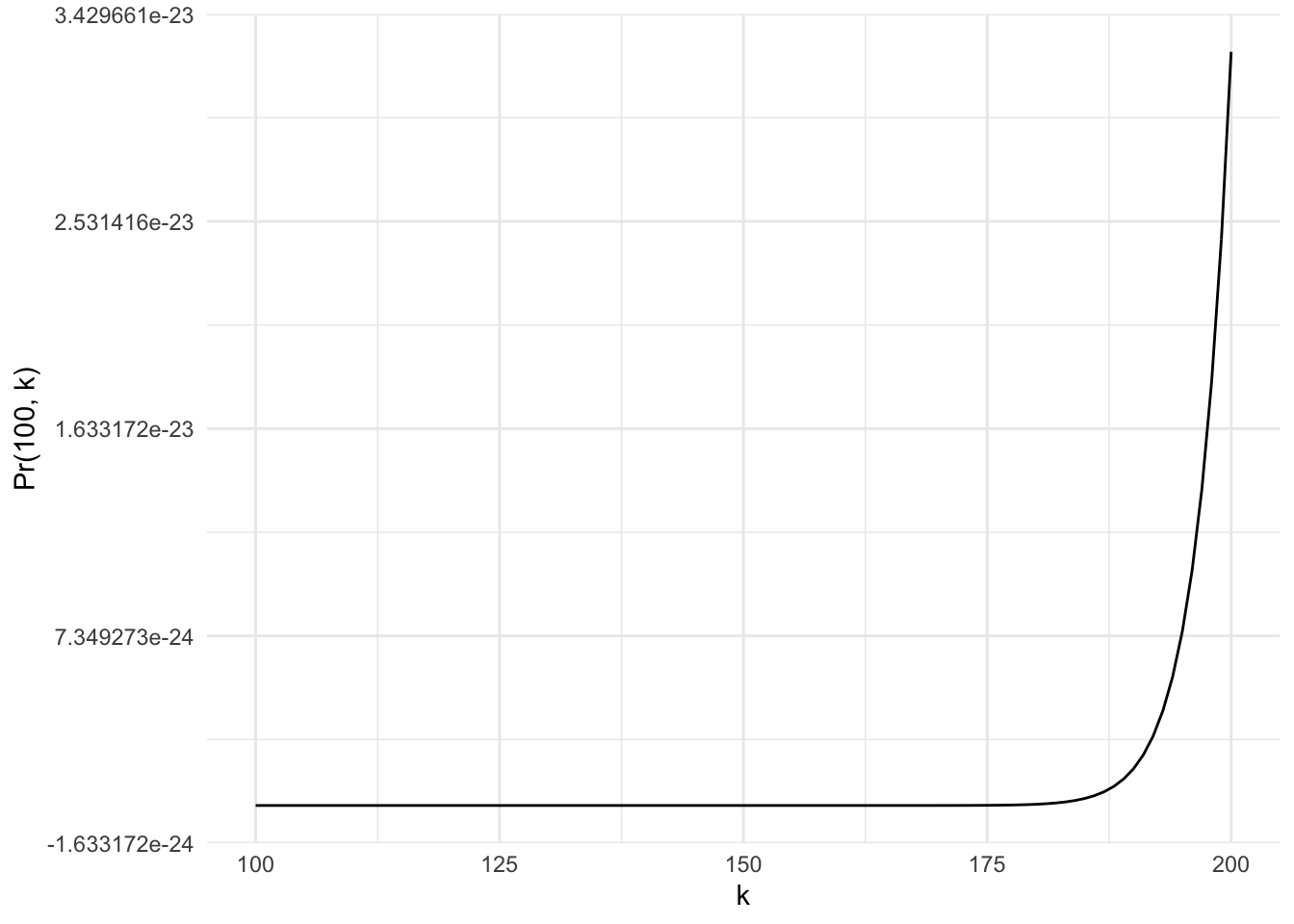

The plot shows that the probability of getting all prisoners at least once even after the warden takes 200 times is so slim that it’s practically 0.

We can extend the possible \(k\) values.

ggplot() +
  xlim(100, 30000) +
  geom_function(fun = Pr) +
  labs(x = "k", y = "Pr(100, k)")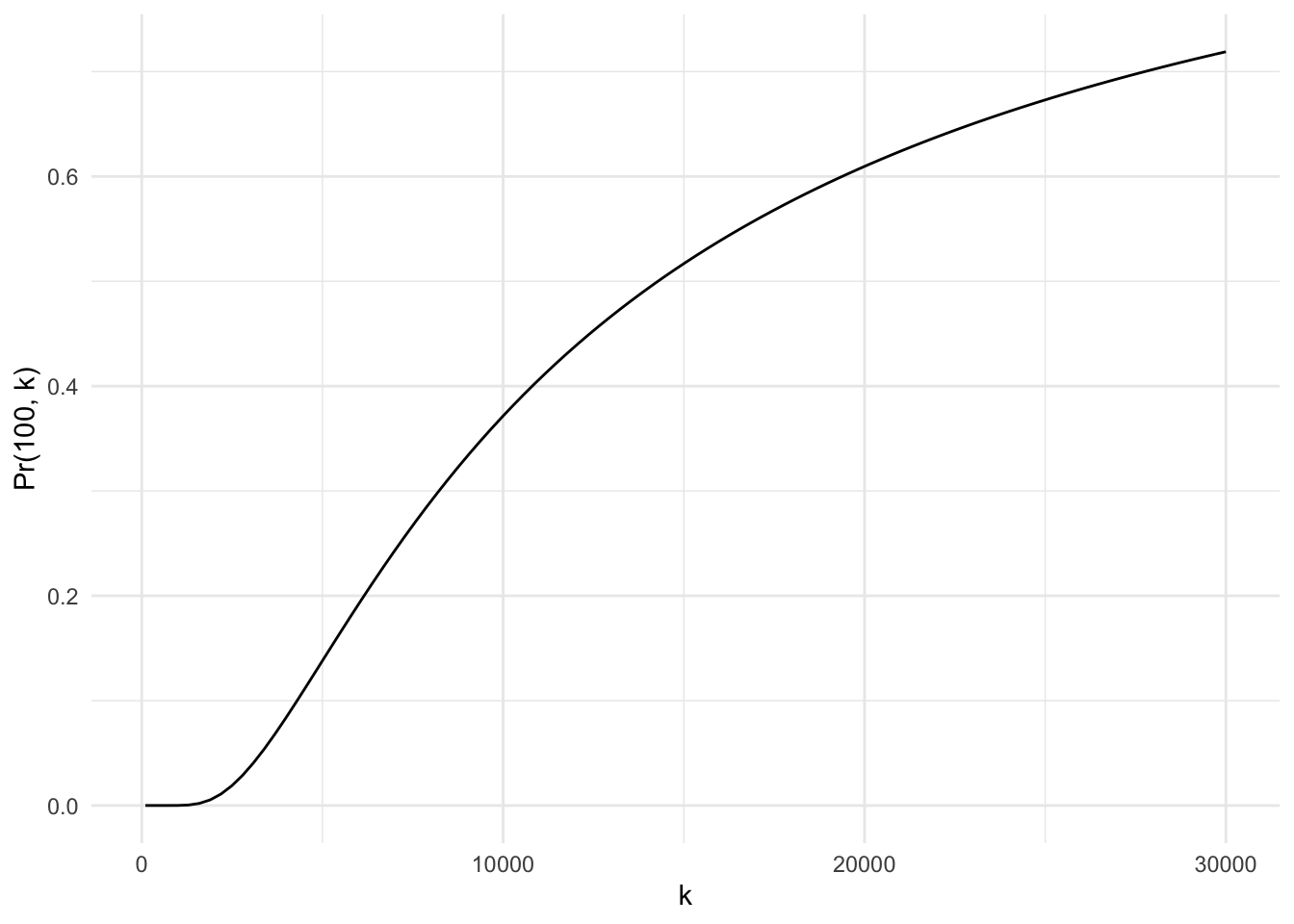

For the probability to reach 10%, the warden needs to take nearly 5,000 times. The probability increases a bit faster once \(k\) exceeds 5,000, but it still takes about 10,000 times before it gets near 40%.

We can also find out the minimum \(k\) that makes the probability greater than 50% (i.e., better than a coin flip).

for (k in seq(100, 30000, 1)) {
  if (Pr(k) >= 0.5) {
    print(paste0("It takes ", k, " times for the probability to reach 50%."))
    break
  }
}

## [1] "It takes 14283 times for the probability to reach 50%."

Assuming that the warden takes 1 prisoner to the room every day, it would take 39.13 years for the odds to be better than a random coin flip.

How about 80% probability?

for (k in seq(100, 50000, 1)) {
  if (Pr(k) >= 0.8) {
    print(paste0("It takes ", k, " times for the probability to reach 80%."))
    break
  }
}

## [1] "It takes 44367 times for the probability to reach 80%."

That’s 121.55 years! If that ever happens, the warden has to be the most dedicated warden in history.

Is it right?

The short answer is: No.

The slightly longer and more informative answer is: No, because this assumption is wrong.

Since the order of the prisoners doesn’t matter, the problem is a combination question. To correctly compute the probability, the order in which the prisoners are taken does matter and it should be a permutation question.

It’s hard to see this logic using a 100-element set, so let’s use a simple 3-element dummy set instead.

Suppose there is a 3-element unique set \(S\), {\(A\), \(B\) \(C\)}.

There are \(\left(\!\!{3\choose 3}\!\!\right) = {{3+3-1}\choose{3}} = {{5}\choose{3}} = 10\) 3-combinations (with repetition) one can draw from the set.

#	3-combinations
1	(\(A\), \(A\), \(A\))
2	(\(A\), \(A\), \(B\))
3	(\(A\), \(A\), \(C\))
4	(\(A\), \(B\), \(B\))
5	(\(A\), \(B\), \(C\))
6	(\(A\), \(C\), \(C\))
7	(\(B\), \(B\), \(B\))
8	(\(B\), \(B\), \(C\))
9	(\(B\), \(C\), \(C\))
10	(\(C\), \(C\), \(C\))

It’s easy to see that among the 10 combinations, only one set, (\(A\), \(B\), \(C\)), includes all 3 unique elements. So the probability is simply \(1/10 = 0.1\).

Alternatively, we can simply plug in \(n=3, k=3\) into the formula.

\[Pr(3,3) = \frac{3!(3-1)!}{(3+3-1)!(3-3)!} = \frac{3!2!}{5!0!} = \frac{3 \times 2 \times 1 \times 2 \times 1}{5 \times 4 \times 3 \times 2 \times 1} = \frac{12}{120} = 0.1\]

Is the probability really 10%? We can run a simulation to find out.

n <- 3
k <- 3
S <- LETTERS[1:n]
sims <- replicate(50000, sample(S, k, replace = TRUE), simplify = FALSE)
(p <- sum(sapply(sims, function(x) length(setdiff(S, x)) == 0))/50000)

## [1] 0.22504

The simulation suggests that 22.5% of the samples have all 3 unique elements in them. That’s a lot higher than the 10% that we’ve computed.

This is because the combination that has all 3 elements is actually more likely to happen in permutations.

The total number of 3-permutations (with repetition) from a 3-element unique set is \(3^3 = 27\). The total number of 3-permutations (without repetition) from the same set is \(3! = 3 \times 2 \times 1 = 6\). Therefore, the probability of a sample set having all 3 elements is \(6/27 \approx 22.2\%\).

One can imagine a frequency multiplier for each one of the 10 possible 3-combinations. This multiplier tells how many permutations a particular combination has. If all combinations have the same multiplier, the probability formula using combination counts would be right. The simple example shows that this is not the case and the combination with all 3 elements must have a greater multiplier than average.

In the table above, we list out all possible 3-combinations. We can also represent each combination by the number of unique elements it has and how many times each unique element occurrs. For example, in (\(A\), \(A\), \(B\)), there are 2 unique elements \(A\) and \(B\). \(A\) occurrs twice and \(B\) once. Let’s denote each unique elements’s frequency in a combination \(m_j\). In the example, \(m_1 = 2\) and \(m_2 = 1\).

One can show that the number of permutations (aka the frequency multiplier) of a \(m\)-element combination is \(\frac{m!}{m_1! \cdot m_2! \cdot ... \cdot m_j!}\), where \(\sum{m_j}=m\)

It’s clear from this formula why the combination having all 3 elements has the greatest frequency multiplier. All combinations have the same numerator \(m!\) while the combination having all 3 elements has the lowest denominator.

This makes me think that our probability formula is vastly underestimating the actual probability. The prisoners might have a shot at this game after all.

Permutation

It’s straightforward to compute the denominator which is the total number of possible permutations. When drawing \(k\) items (with repetition) from a unique \(n\)-element set, the total number of permutations is simply \(n^k\) (each item of the \(k\) items can be any one of the \(n\) elements from the set).

The numerator isn’t so easy to compute. One needs to use the inclusion-exclusion principle.

First of all, the number of permutations that have all elements from the unique set is equal to the total number of possible permutations minus the number of permutations that miss at least one element from the unique set.

Let’s denote set of all \(k\)-permutations that miss element \(i\) as \(M_i\). Therefore, \(M_1\) include all \(k\)-permutations that miss element \(1\), and so on.

The numerator we’re interested in can be computed as the following.

\[n^k-(\]

\[|M_1| + |M_2| + ... + |M_n|\] \[- |M_1 \cap M_2| - ... - |M_{n-1} \cap M_n|\] \[+ |M_1 \cap M_2 \cap M_3| + ... + |M_{n-2} \cap M_{n-1} \cap M_n|\] \[- ... - ...\] \[+ (-1)^n|M_1 \cap M_2 \cap ... \cap M_n|)\]

This can be simplified to

\[n^k - ((n-1)^k{{n}\choose{1}} - (n-2)^k{{n}\choose{2}} + ... + (-1)^{n-1}(n-n)^k{{n}\choose{n}})\]

Since \(n^k\) can be written as \((n-0)^k{{n}\choose{0}}\), the formula can be simplified.

\[\sum_{j=0}^{n} (-1)^{j} (n-j)^k {{n}\choose{j}}\]

For example, when \(n=3\) and \(k=3\),

\[\sum_{j=0}^{3} (-1)^{j} (3-j)^3 {{3}\choose{j}}\] \[=3^3 - 2^3{{3}\choose{1}} + 1^3{{3}\choose{2}} - 0 = 27 - 8 \cdot 3 + 1 \cdot 3 = 6\]

Now we have both the numerator and denominator, we can compute the probability function.

\[Pr(n,k) = \frac{\sum_{j=0}^{n} (-1)^{j} (n-j)^k {{n}\choose{j}}}{n^k}\] \[=\sum_{j=0}^{n} (-1)^{j} (\frac{n-j}{n})^k {{n}\choose{j}}\]

We can now plot the probability function for \(n=100\) and \(100 \leq k \leq 200\).

Pr <- function(n, k) {
  out <- vector("numeric", n+1)
  for (j in seq(0, n, 1)) {
    out[j+1] <- (-1)^j * ((n-j)/n)^k * choose(n, j)
  }
  max(0, sum(out))
}
Pr_100 <- function(k) {
  sapply(k, function(k) Pr(100, k))
}
ggplot() +
  xlim(100, 200) +
  geom_function(fun = Pr_100) +
  labs(x = "k", y = "Pr(100, k)")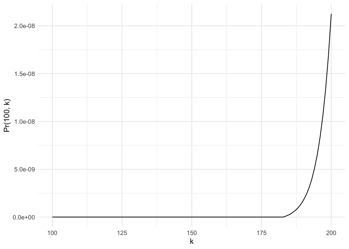

The probability of getting all prisoners taken at least once after 200 times is still very slim and effectively 0. What about higher \(k\) values?

ggplot() +
  xlim(100, 1000) +
  geom_function(fun = Pr_100) +
  labs(x = "k", y = "Pr(100, k)")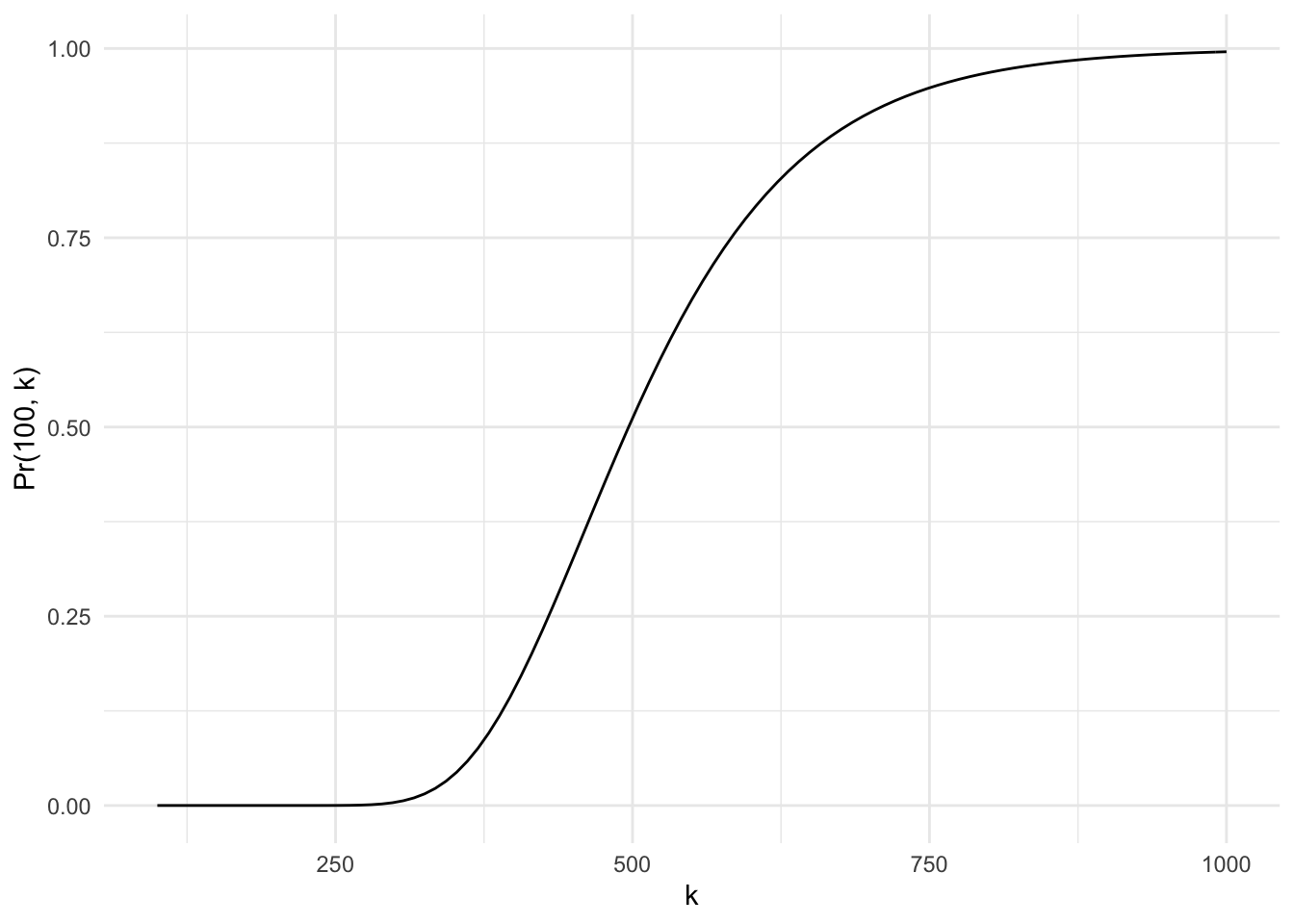

Now we see that the probability starts to increase fairly quickly when \(k\) exceeds 400. It also reaches its peak roughly when \(k\) approaches 800.

We can also compute the minimum \(k\) value for the probability to reach 50%.

for (k in seq(100, 1000, 1)) {
  if (Pr_100(k) >= 0.5) {
    print(paste0("It takes ", k, " times for the probability to reach 50%."))
    break
  }
}

## [1] "It takes 497 times for the probability to reach 50%."

It takes just shy of 500 times to get even odds. How about 80%?

for (k in seq(100, 1000, 1)) {
  if (Pr_100(k) >= 0.8) {
    print(paste0("It takes ", k, " times for the probability to reach 80%."))
    break
  }
}

## [1] "It takes 609 times for the probability to reach 80%."

It takes 112 more tries for the probability to get to 80%. Similarly, we can compute that it takes 754 tries for the probability to reach 95%.

We can use simulation to confirm if the probability formula is correct.

Sim <- function(k, n) {
  S <- seq(1, n, 1)
  sims <- replicate(1000, sample(S, k, replace = TRUE), simplify = FALSE)
  sum(sapply(sims, function(x) length(setdiff(S, x)) == 0))/1000
}
Sim_100 <- function(k, n) {
  sapply(k, function(k) Sim(k, n))
}
ggplot() +
  xlim(100, 1000) +
  geom_function(fun = Pr_100) +
  geom_function(fun = Sim_100, args = list(n = 100), color = "red") +
  labs(x = "k", y = "Pr(100, k)")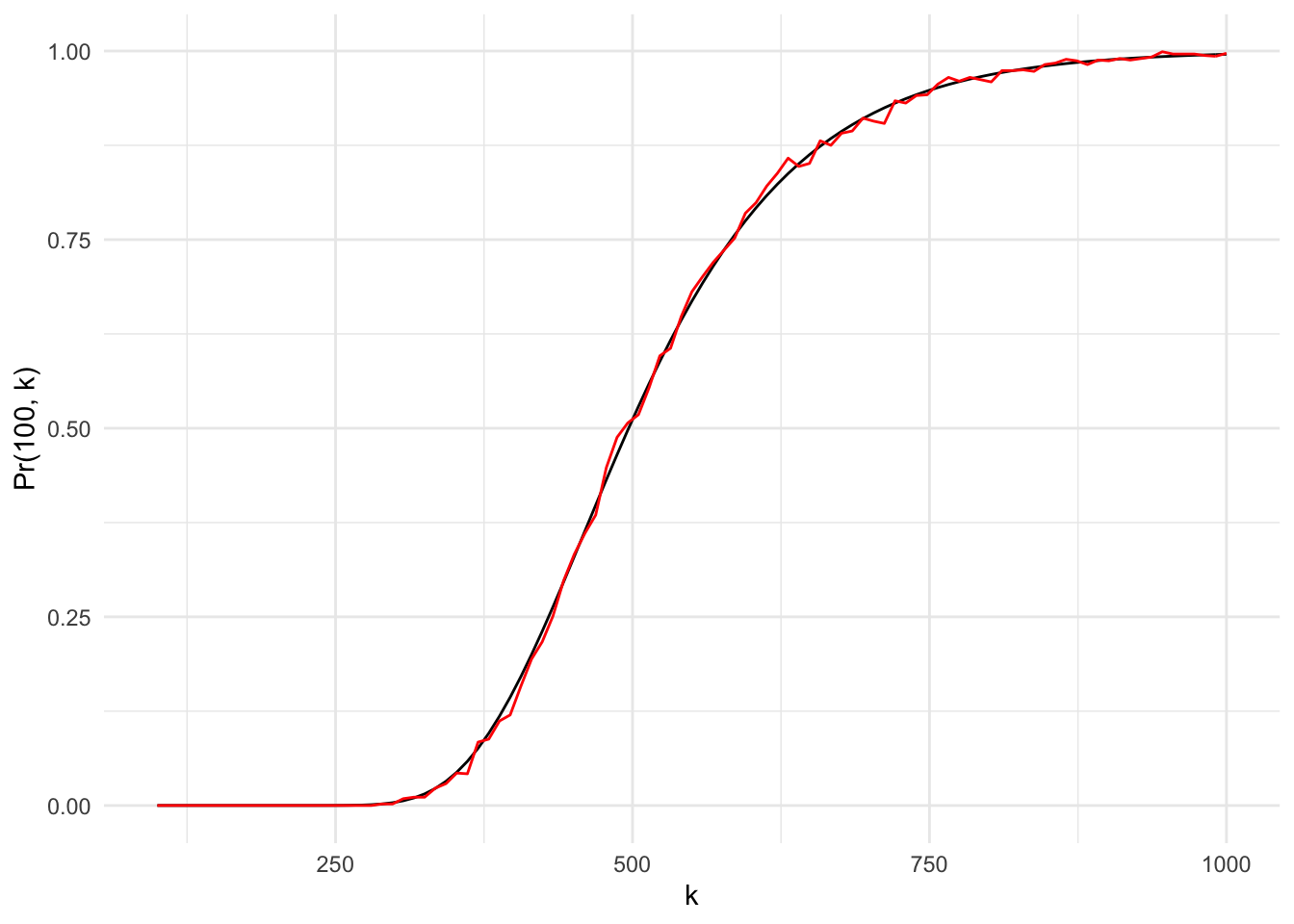

The simulation produces very simliar probability curve to the probability function.

Now it becomes a collective bargaining problem. All prisoners need to agree on a particular probability threshold and compute the necessary tries to get to that probability. If they assume that the warden only takes one prisoner every day, then the number of tries equals the number of days they need to wait before someone makes the assertion and all hope for the best.