The journey of discovering four-of-a-kind in a standard deck of cards ·

I was reading Prof David Pollard’s Probability Theory with Applications. Chapter 1 of the notes has a brief introduction of probability. Example 1.2 in the chapter asks a very simple question.

What is the probability that a hand of 5 cards (from a standard deck) contains four-of-a-kind?

The technique Prof Pollard used to solve the problem is to break the event (that is, a hand of 5 cards contains four-of-a-kind) into disjoint symmetric pieces (i.e., subevents). The disjointedness indicates that those subevents cannot occur at the same time. The symmetry is not guaranteed (i.e., mutually exclusive subevents don’t necessarily occur at the same frequency or probability), but is usually present in many probability problems.

A standard deck of cards has 13 ranks (i.e., from ace to king). Therefore there are 13 mutually exclusive subevents of having four-of-a-kind in 5 cards (i.e., four aces, four twos, …, up to four kings).

I use $P(k \geq 1, n=5)$ to denote the probability of having any four-of-a-kind in a 5-card hand.

\[ P(k \geq 1, n=5)=\sum_{i=1}^{13} P(F_{i}) \]

where $F_{i}$ corresponds to a subevent of having a particular four-of-a-kind ranging from ace to king. Since those subevents are disjoint, the probability of the overall event is the sum of the probabilities of those subevents. Furthermore, in a standard deck, the probability of having a four-of-a-kind of any rank should be the same as any other rank, that is, $P(F_1) = P(F_2) = ... = P(F_{13})$.

\[ P(k \geq 1, n=5) = \sum_{i=1}^{13} P(F_{i}) = 13 \times P(F_1) \]

Here we use $P(F1)$ as a placeholder. One can substitute it with any other subevent $F_i$.

We can further break the subevent $F_1$ (that is, having four aces in 5 cards) into 5 disjoint and symmetric sub-subevents. For a hand of a 5 cards to have 4 aces, there must be one other card that’s not an ace. This “residual” card can be at any position (i.e., from 1st to 5th) in the hand. Those 5 different positions constitute 5 disjoint sub-subevents. Conceptually it’s straightforward to deduce that those sub-subevents have the same probability of happening (i.e., symmetry).

\[ P(F_1) = \sum_{j=1}^{5} P(F_{1, j}) \]

where $F_{1, j}$ refers the sub-subevent whereby there are 4 aces and 1 residual card in a 5-card hand and the residual card is at the position $j$.

Since we’ve already established that $P(F_{1,1}) = P(F_{1,2}) = P(F_{1,3}) = P(F_{1,4}) = P(F_{1,5})$, we can simplify the equation.

\[ P(F_1) = \sum_{j=1}^{5} P(F_{1, j}) = 5 \times P(F_{1, 1}) \]

We can now work out the probability of $F_{1,1}$ which corresponds to a particular chain of actions.

Draw a non-ace card from a standard deck
Draw an ace from the rest of the deck
Draw another ace from the rest of the deck
Draw yet another ace from the rest of the deck
Draw the final ace from the rest of the deck

\[ P(F_{1,1}) = P(A_1) \cdot P(A_2) \cdot P(A_3) \cdot P(A_4) \cdot P(A_5) \]

where $A_i$ corresponds to the actions mentioned above in the numbered list.

$P(A_1) = \frac{48}{52}$ because there are 48 non-ace cards in the deck.
$P(A_2) = \frac{4}{51}$ because there are 4 aces in the rest of the deck which now has 51 cards.
$P(A_3) = \frac{3}{50}$ because there are now 3 aces in the remaining 50-card deck.
$P(A_4) = \frac{2}{49}$ because there are now 2 aces left in the remaining 49-card deck.
$P(A_5) = \frac{1}{48}$ because there’s only 1 ace left in the remaining 48-card deck.

Therefore,

\[ P(F_{1,1}) = \frac{48}{52} \cdot \frac{4}{51} \cdot \frac{3}{50} \cdot \frac{2}{49} \cdot \frac{1}{48} \]

Putting all these steps together, we can arrive at the final conclusion.

\[ \begin{aligned} P(k \geq 1, n=5) &= \sum_{i=1}^{13} P(F_{i}) = 13 \times P(F_1) \\ &= 13 \times 5 \times P(F_{1, 1}) \\ &= 13 \times 5 \times \frac{48}{52} \cdot \frac{4}{51} \cdot \frac{3}{50} \cdot \frac{2}{49} \cdot \frac{1}{48} \\ &= \frac{1}{4165} \\ &\approx 0.00024 \end{aligned} \]

The probability is quite low. On average, there is only 1 such hand in 4,000+ hands.

This reasoning emphasizes on breaking the event-of-interest into cascading mutually exclusive (i.e., disjoint) subevents (imagine a tree of subevents). Those subevents on the same level usually have symmetry among them so that only one of them is needed for subsequent steps.

An alternative approach

The most straightforward (at least to me) approach of computing a probability is to count the number of scenarios that match the event-of-interest and the total number of possible scenarios.

\[ P(\text{event}) = \frac{\text{# of scenarios that match event}}{\text{total # of possible scenarios}} \]

In this case, the event-of-interest is having four-of-a-kind in a 5-card hand. The total number of possible scenario (i.e., the denominator) is the total # of possible 5-card hands. This is easy to compute using combinatorics.

\[ \text{total # of 5-card hands} = \binom{52}{5} = \frac{52!}{5! \cdot 47!} = 2,598,960 \] A 5-card hand that contains four-of-a-kind can be thought of the combination of two elements.

Choose 1 rank from the total 13 ranks to the kind of the four-of-a-kind.
Choose 1 residual card from the remaining deck after the four-of-a-kind has been drawn.

\[ \begin{aligned} \text{# of scenarios that match event} &= \binom{13}{1} \times \binom{52-4}{5-4} \\ &= \binom{13}{1} \times \binom{48}{1} = 13 \times 48 = 624 \end{aligned} \]

There are 624 different 5-card hands that contain four-of-a-kind. So the probability of having four-of-a-kind in any 5-card hand is

\[ \begin{aligned} P(k \geq 1, n=5) &= \frac{\text{# of scenarios that match event}}{\text{total # of possible scenarios}} \\ &= \frac{624}{2,598,960} = \frac{1}{4165} \approx 0.00024 \end{aligned} \]

First attempt to generalize

After solving the initial question, I immediately wanted to know what if we change the number of cards in the hand. A natural candidate for the next enquiry is a 7-card hand (which is commonly used in games like Text Hold’em). Following the logic above, it’s very straightforward to compute the probability.

\[ \begin{aligned} P(k \geq 1, n=7) &= \frac{\binom{13}{1} \cdot \binom{48}{3}}{\binom{52}{7}} \\ &= \frac{13 \cdot \frac{48!}{3! \cdot 45!}}{\frac{52!}{7! \cdot 45!}} = \frac{13 \cdot 48! \cdot 7!}{3! \cdot 52!} \\ &= \frac{13 \cdot 7 \cdot 6 \cdot 5 \cdot 4}{52 \cdot 51 \cdot 50 \cdot 49} = \frac{1}{595} \approx 0.00168 \end{aligned} \] The probability of having four-of-a-kind has increased significantly from 0.024% to 0.17% as the extra 2 cards in the hand should help increase the chance of having a four-of-kind, but the overall probability is still very low (there’s a reason why four-of-a-kind is a very strong hand in Texas Hold’em).

It’s tempting to generalize the formula.

\[ \begin{aligned} P(k \geq 1, n) &= \frac{\binom{13}{1} \cdot \binom{48}{n-4}}{\binom{52}{n}} \\ &= \frac{13 \cdot \frac{48!}{(n-4)! \cdot (52-n)!}}{\frac{52!}{n! \cdot (52-n)!}} \\ &= \frac{13 \cdot 48! \cdot n!}{(n-4)! \cdot 52!} \\ &= \frac{13 \cdot n \cdot (n-1) \cdot (n-2) \cdot (n-3)}{52 \cdot 51 \cdot 50 \cdot 49} \end{aligned} \]

I plot the results of $n$ ranging from 0 to 28 below.

prob1 <- function(n) {
  choose(13, 1) * choose(48, n-4) / choose(52, n)
}
df1 <- tibble(
  n = 0:52,
  p = map_dbl(n, prob1)
)
df1 %>% 
  filter(n <= 28) %>%
  ggplot(aes(x = n, y = p)) +
    geom_point() +
    geom_linerange(aes(ymin = 0, ymax = p)) +
    scale_x_continuous(breaks = seq(0, 28, 1)) +
    scale_y_continuous(label = percent)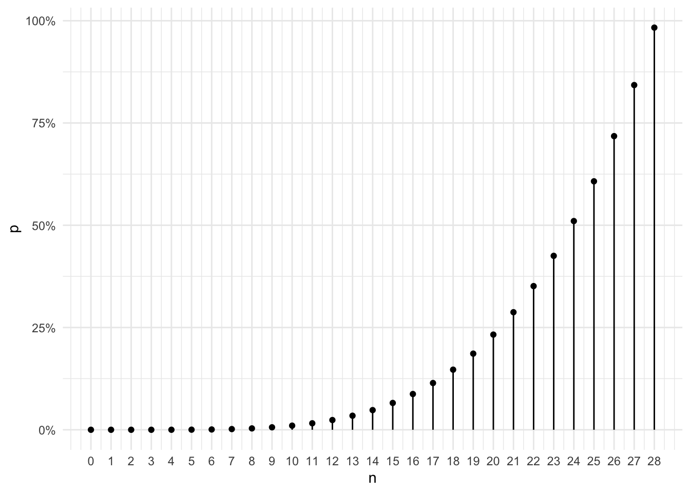

Observations:

When $n$ is smaller than 4 (i.e., 0, 1, 2, or 3), the probability of having four-of-a-kind is 0. This should be so obvious since by definition four-of-a-kind requires 4 cards. The formula does produce 0 for $n$ smaller than 4 because $n \cdot (n-1) \cdot (n-2) \cdot (n-3)$ in the numerator equals 0 when $n$ is 0, 1, 2, or 3.
The probability is a quartic function (i.e., a polynomial of degree four) of $n$. When $n$ is small (such as 5), the probability is very small. But the probability increases very fast when $n$ increases.

One thing I noticed on the chart is that the probability of having four-of-a-kind in a 28-card hand (i.e., the last point on the chart) is very close to 1. Given the quartic nature of the function, it is bound to exceed 1 when $n$ exceeds 28. In fact, $P(29) = 1.14$. A more extreme case would be $n=52$. Such a 52-card hand is basically the whole deck and the probability of having four-of-kind in the hand is 1. But according to the formula, $P(52) = 13$ which is much greater than 1 and doesn’t make sense.

Duplication and overcounting

So apparently the generalized formula is wrong, or at least no applicable to all possible $n$ values. The trouble is duplication of scenarios which results in overcounting and overestimation of the probability.

To see this, take the case whereby $n=8$.

The numerator is computed as $\binom{13}{1} \cdot \binom{52-4}{n-4} = \binom{13}{1} \cdot \binom{48}{4} = 2,529,540$. This can be thought as a 2-step process. (i), 4 cards of a kind are drawn. Since there are 13 ranks in a deck, there are $\binom{13}{1} = 13$ ways of drawing those 4 cards. (ii), next $n-4=4$ cards are drawn from the rest of the deck which now has $52-4=48$ cards. There are $\binom{48}{4} = 194,580$ ways to draw those 4 residual cards. Those two steps are independent of each other, so the total number of scenarios is the product of those two $13 \times 194,580 = 2,529,540$.

\[ P(k \geq 1, n=8) = \frac{2,529,540}{\binom{52}{8}} = \frac{2,529,540}{752,538,150} = \frac{2}{595} \approx 0.0033613 \]

This logic is flawed because there are actually duplication of the same scenarios. For example, let’s say ace is the rank drawn in the first step. That is, the first step draws 4 aces from the deck. When one draws another 4 cards from the rest of the deck, it’s possible to draw another four-of-a-kind (albeit a different kind than ace). In fact, there are $\binom{12}{1} = 12$ ways to draw another four-of-a-kind in the second step. Drawing 4 aces in the first step and drawing 4 twos in the second step makes the 8-card hand $\{ace, ace, ace, ace, 2, 2, 2, 2\}$. One can reverse the order of the two steps to reach the same hand (remember that the order of the cards in the hand doesn’t matter). If 4 twos are drawn in the first step and 4 aces are drawn in the second, the hand is $\{2, 2, 2, 2, ace, ace, ace, ace\}$ which is effectively the same hand. Therefore, there are some duplication of scenarios in the numerator $2,529,540$ and this duplication makes the probability higher than it really is.

Now the question becomes how to quantify the duplication and correct the overcounting.

For this particular case of $n=8$. The duplication occurs when two four-of-a-kind sets are drawn in different orders in the two-step process (i.e., aces before twos vs. twos before aces). There are 13 ways to draw the first four-of-a-kind and for each of those four-of-a-kind, there are 12 ways to draw the second four-of-a-kind, so there are in total $13 \times 12 = 156$ scenarios that have two four-of-a-kind sets in the numerator. Since there are only two sets of four-of-a-kind, the duplication is precisely double-counting (i.e., aces-and-twos and twos-and-aces are the same). So to correct for the duplication, I need to subtract $156/2=78$ scenarios from the numerator.

I use $P'()$ to denote the corrected probability formula.

\[ P'(k \geq 1, n=8) = \frac{2,529,540-78}{\binom{52}{8}} = \frac{2,529,462}{752,538,150} \approx 0.0033612 \]

The corrected probability is very close to the previous one because the magnitude of the duplication is very limited (i.e., 78 scenarios in 2.5+ million).

Second attempt to generalize

In the previous section I took the approach of subtracting duplicated scenarios from total number of scenarios (which is computed using the two-step process) to arrive at the right probability of having four-of-a-kind in an 8-card hand. So naturally I wanted to explore the possibility of generalizing this approach to any $n \in [0, 52]$.

To recap, I have solved the probability of having four-of-a-kind in three situations so far.

When $0 \leq n \leq 3$, $\underset{0 \leq n \leq 3}P(k \geq 1, n) = 0$.
When $4 \leq n \leq 7$, $\underset{4 \leq n \leq 7}P(k \geq 1, n) = \frac{\binom{13}{1} \cdot \binom{48}{n-4}}{\binom{52}{n}}$.
When $8 \leq n \leq 11$, $\underset{8 \leq n \leq 11}P(k \geq 1, n) = \frac{\binom{13}{1} \cdot \binom{48}{n-4} - \binom{13}{2} \cdot \binom{44}{n-8}}{\binom{52}{n}}$

My first attempt to generalize only works in the second case. When $4 \leq n \leq 7$, $0 \leq n-4 \leq 3$ and there are no four-of-a-kind in all $\binom{48}{n-4}$ residual card scenarios (hence no risk of duplication and overcounting). Conveniently most poker hands (e.g., 5-card hand and 7-card hand) are within this case and the naive generalized formula works just fine.

The formula in the third case above builds upon the naive generalized formula by correcting the numerator (i.e., subtracting the number of duplicated scenarios). The correction term $\binom{13}{2} \cdot \binom{44}{n-8}$ is itself computed following a two-step logic. (i), there are $\binom{13}{2} = 78$ ways of drawing 2 sets of four-of-a-kind from 13 ranks included in a standard deck of cards. (ii), for each of those 78 combinations of 2 sets of four-of-a-kind, there are $\binom{44}{n-8}$ ways to draw the residual $n-8$ (remember that two sets of four-of-a-kind have been drawn) cards. Since all of those $\binom{13}{2} \cdot \binom{44}{n-8}$ scenarios appear twice in the naive generalied formula’s numerator $\binom{13}{1} \cdot \binom{48}{n-4}$, they need to be subtracted once to arrive at the right numerator. The reason why this corrected generalized formula only works for $8 \leq n \leq 11$ is that $n-8 \geq 4$ when $n \geq 12$ and it would incur more unaccounted duplication.

My second attempt to generalize the formula for any $n$ focuses on finding a way to compute the duplication as $n$ increases and subtract them from the original numerator $\binom{13}{1} \cdot \binom{48}{n-4}$.

If the double-counting problem (i.e., having 2 sets of four-of-a-kind) can be mitigated using the correction term $\binom{13}{2} \cdot \binom{44}{n-8}$, it seems promising to modify it to $\binom{13}{3} \cdot \binom{40}{n-12}$ to correct for the triple-counting (i.e., having 3 sets of four-of-a-kind) problem.

I use $k$ to represent the variable that corresponds to the maximum number of sets of four-of-a-kind in an $n$-card hand. It’s not difficult to deduce that $k \in [0, \lfloor n/4 \rfloor]$.

When $0 \leq n \leq 3$, $k = \lfloor n/4 \rfloor = 0$.
When $4 \leq n \leq 7$, $k \in [0, \lfloor n/4 \rfloor] = [0, 1]$.
When $8 \leq n \leq 11$, $k \in [0, \lfloor n/4 \rfloor] = [0, 2]$.
…
When $n = 52$, $k \in [0, \lfloor n/4 \rfloor] = [0, 13]$.

When $k$ sets of four-of-a-kind are possible in an $n$-card hand, there are $\binom{13}{k} \cdot \binom{52-4k}{n-4k}$ scenarios of such unique $n$-card hands. Each of those unique hand is included in the original $\binom{13}{1} \cdot \binom{48}{n-4}$ $k$ times. So to correct the duplication, $(k-1) \cdot \binom{13}{k} \cdot \binom{52-4k}{n-4k}$ scenarios need to be subtracted.

\[ P'(k \geq 1, n) = \frac{\binom{13}{1} \cdot \binom{48}{n-4} - \sum\limits_{k=2}^{13} (k-1) \cdot \binom{13}{k} \cdot \binom{52-4k}{n-4k}}{\binom{52}{n}} \]

I plot the results below using the new generalized formula.

prob2 <- function(n) {
  start = choose(13, 1) * choose(48, n-4)
  correction = sum(
    map_dbl(seq(2, 13, 1), ~(.x - 1) * choose(13, .x) * choose(52-4*.x, n-4*.x))
  )
  (start - correction) / choose(52, n)
}
df2 <- tibble(
  n = 0:52,
  p = map_dbl(n, prob2)
)
df2 %>%
  filter(n <= 28) %>%
  ggplot(aes(x = n, y = p)) +
    geom_point() +
    geom_linerange(aes(ymin = 0, ymax = p)) +
    scale_x_continuous(breaks = seq(0, 28, 1)) +
    scale_y_continuous(label = percent, limits = c(0, 0.6))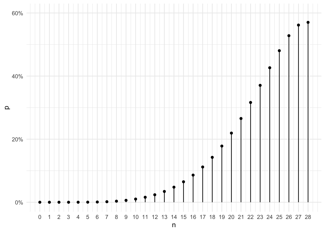

Comparing this chart to figure 1 shows some differences.

The corrections seem to have little impact on the probabilities when $n$ is small (i.e., $n ).
For larger $n$s, the corrections have material impact. $P'(28)$ is close to 60% rather than 100%.

I plot the two figures together to show the differences more clearly.

df1n2 <- bind_rows(
  mutate(df1, version = "original"),
  mutate(df2, version = "corrected")
) %>%
  mutate(version = factor(version, levels = c("original", "corrected")))
df1n2 %>%
  filter(n <= 28) %>%
  ggplot(aes(x = n, y = p)) +
    geom_point(aes(color = version)) +
    scale_x_continuous(breaks = seq(0, 28, 1)) +
    scale_y_continuous(label = percent) +
    theme(legend.position = "top")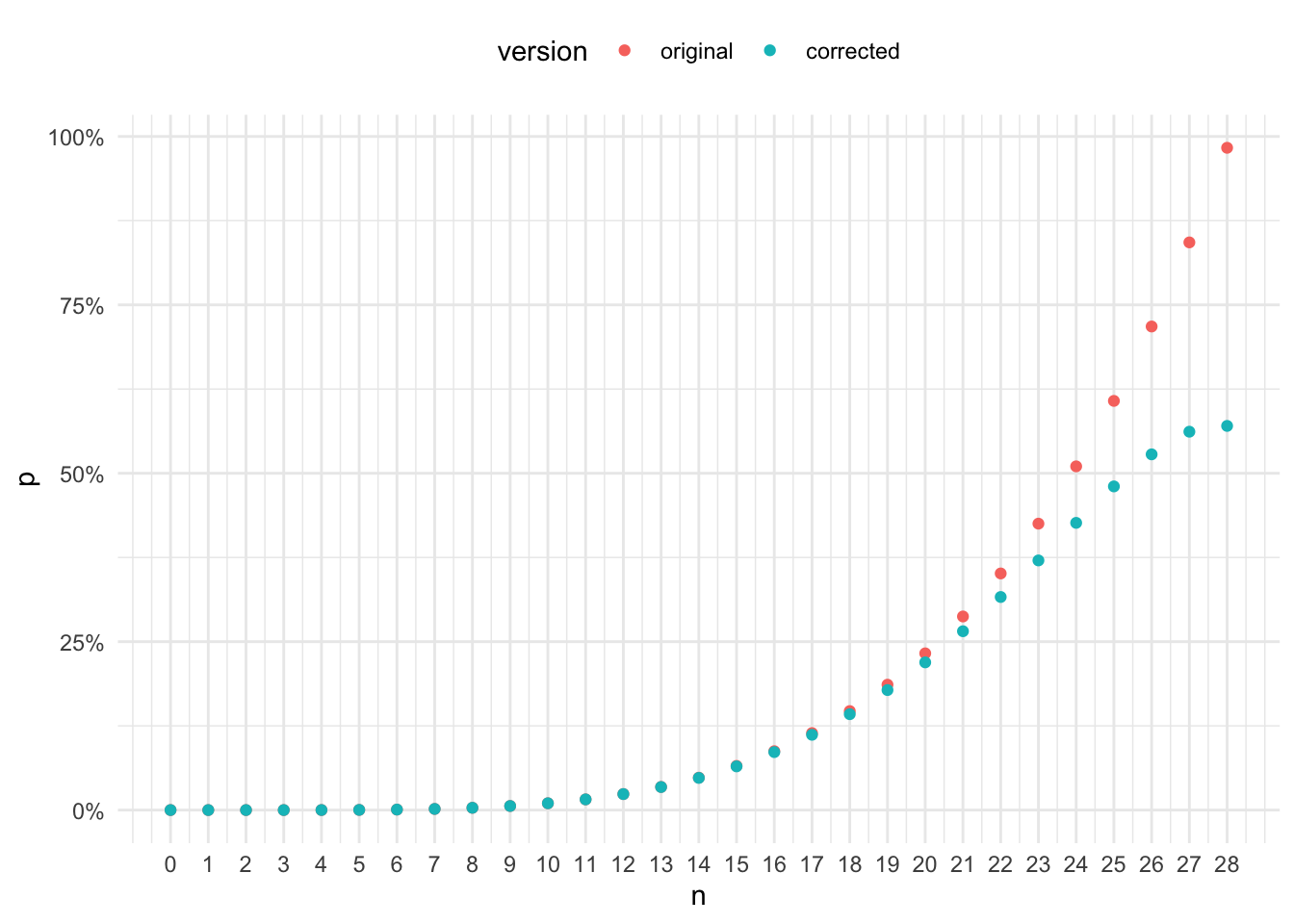

The differences are rather small when $n \leq 20$. They start to emerge and quickly increase when $n > 20$. The shape of the corrected formula curve looks S-shape rather than quartic or exponential. In fact, if I expand the x-axis a bit to include $n \in [29, 32]$, it shows that the corrected formula starts to produce lower probabilities.

df1n2 %>%
  filter(n <= 32) %>%
  ggplot(aes(x = n, y = p)) +
    geom_point(aes(color = version)) +
    geom_hline(yintercept = 0, linetype = "dashed") +
    geom_hline(yintercept = 1, linetype = "dashed") +
    geom_vline(xintercept = 28, color = "red", linetype = "dashed") +
    scale_x_continuous(breaks = seq(0, 32, 1)) +
    scale_y_continuous(label = percent) +
    theme(legend.position = "top")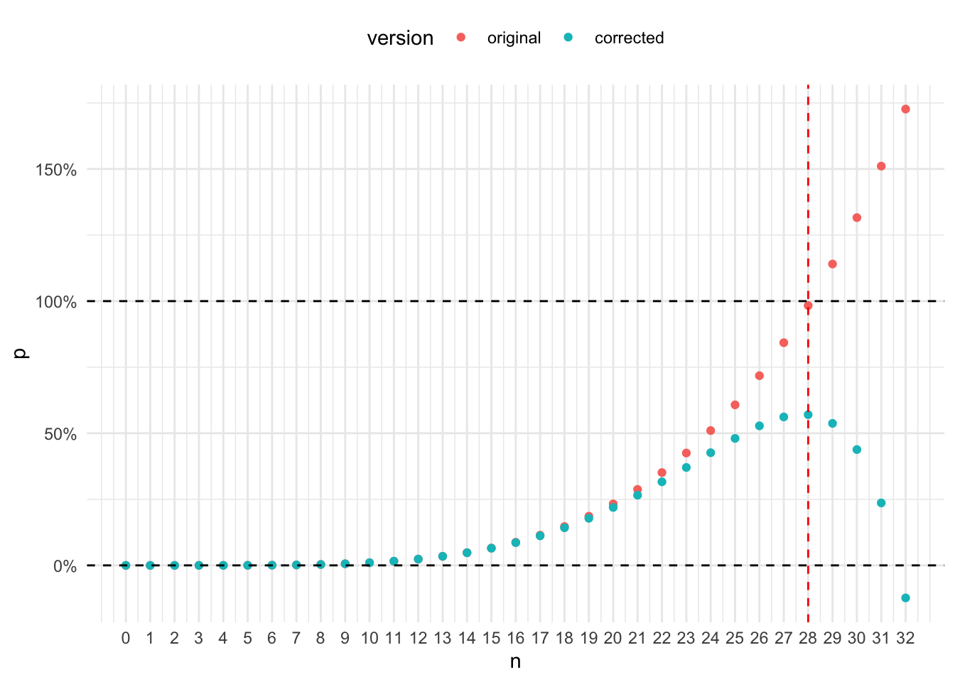

The area between the two black horizontal dashed lines are sensible probabilities (i.e., $[0, 1]$). The chart above shows that both the original formula and the corrected one produce probabilities outside of the sensible range. This means that neither formula is correct. The original formula overcounts and it seems that the corrected formula undercounts (or put it another way, it overcorrects).

I take a closer look at the sum of correction terms $\sum\limits_{k=2}^{13} (k-1) \cdot \binom{13}{k} \cdot \binom{52-4k}{n-4k}$. When $k$ is small, the correction term increases very quickly when $n$ increases because there are much more scenarios of $k$ sets of four-of-a-kind in a large $n$-card hand. Then correction terms of different $k$ start to have large amount of duplication (e.g., 2 sets of four-of-a-kind vs. 3 sets of four-of-a-kind). Since duplication between correction terms are not accounted, the sum of correction terms overcorrects and make the probability result underestimated. Thus, in the attempt to correct duplication in the first term $\binom{13}{1} \cdot \binom{48}{n-4}$, I created another duplication problem in the correction terms. The problem is small when $n$ is small, but grows very quickly when $n$ increases (even pushed the probability below 0 when $n=32$).

The learning from the second attempt to generalize:

The true probability is probably between the original and the corrected formula.
The correction (from the $\binom{13}{1} \cdot \binom{48}{n-4}$ scenarios) approach is conceptually difficult because it’s hard to cleanly separate duplication to mutually exclusive collectively exhaustive (MECE) partitions.

The learning prompted me to try out an approach of addition (i.e., enumeration of categories of scenarios) rather than subtraction (i.e., correction from original scenarios).

Simulation results

Before I dive into my third attempt to generalize, I “computed” the probability result using simulations. This is a totally acceptable way of solving problems. Sometimes closed form formulas just can’t be found to solve a problem. Although it lacks the beauty of pure logical deduction, but it’s a very practical way of problem solving (or at least finding an approximate answer to the problem). Since the probability of four-of-a-kind should be very small when $n$ is small, I need to run the simulation a large number of times to get an accurate estimate (that’s really what it is, not an answer, but an estimate) of the probability.

# create a standard deck
create_a_deck <- function(randomize = TRUE) {
  ranks <- c(
    "ace" = 1L,
    "2" = 2L,
    "3" = 3L,
    "4" = 4L,
    "5" = 5L,
    "6" = 6L,
    "7" = 7L,
    "8" = 8L,
    "9" = 9L,
    "10" = 10L,
    "jack" = 11L,
    "queen" = 12L,
    "king" = 13L
  )
  suits <- c("club", "diamond", "spade", "heart")
  R <- length(ranks)
  S <- length(suits)
  D <- R*S
  deck <- vector(mode = "list", length = D)
  for (i in seq_along(suits)) {
    for (j in seq_along(ranks)) {
      id <- (i-1) * R + j
      deck[[id]] <- list(
        id = id,
        suit = suits[i],
        rank = ranks[j]
      )
    }
  }
  if (randomize) {
    deck <- deck[sample(1:D, replace = FALSE)]
  }
  return(deck)
}

# function to draw n cards from a deck d
draw_cards <- function(d, n) {
   d[sample(1:length(d), size = n, replace = FALSE)]
}
# test if a hand of cards had any four-of-a-kind
has_foak <- function(cards) {
  any(table(map_int(cards, pluck, "rank")) >= 4)
}
# draw n cards and test if there are any four-of-a-kind in the hand
one_draw <- function(d, n) {
  cards <- draw_cards(d, n)
  has_foak(cards)
}

ns <- seq(0, 52, 1)
sim_res <- vector(mode = "list", length = length(ns))
deck <- create_a_deck(randomize = FALSE)
df.sim <- cache_rds({
  set.seed(42)
  for (i in seq_along(ns)) {
    sim_res[[i]]  <- tibble(
      n = ns[i],
      p = mean(
        simplify(
          mclapply(
            1:1e6,
            function(x) { one_draw(d = deck, n = ns[i]) },
            mc.cores = 8
          )
        )
      )
    )
  }
  bind_rows(sim_res)
}, clean = FALSE)

Here I plot the simulation results for $n \in [0, 53]$.

df.sim %>%
  ggplot(aes(x = n, y = p)) +
    geom_point() +
    geom_linerange(aes(ymin = 0, ymax = p)) +
    scale_x_continuous(breaks = seq(0, 50, 5)) +
    scale_y_continuous(label = percent)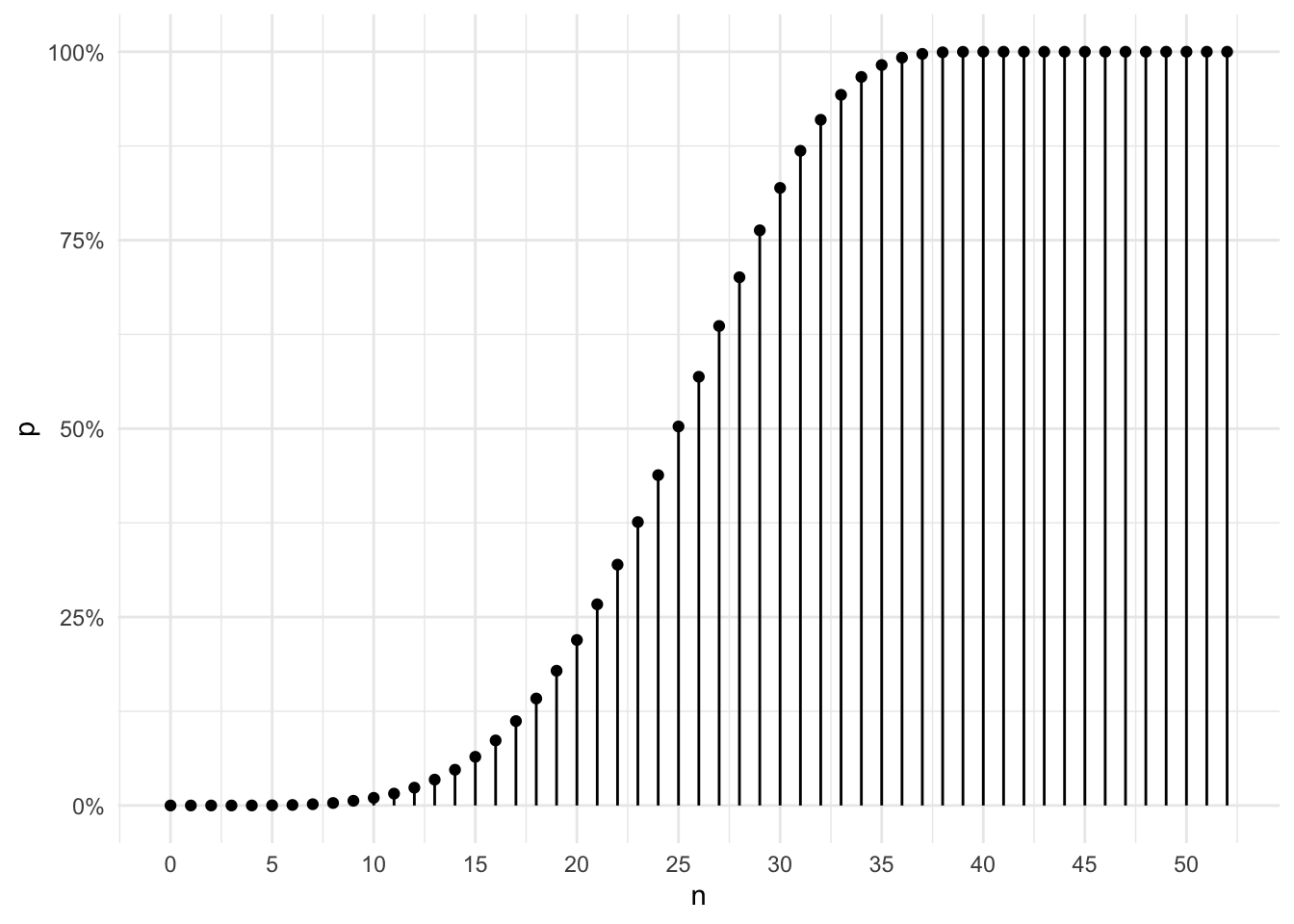

The results are bounded within the $[0, 1]$ range. The curve has an S-shape which makes sense.

When $n \leq 3$, the probability of having four-of-a-kind is 0.
When $n$ is small (i.e., $4 \leq n \leq 10$), the probability of having four-of-a-kind is very small (i.e., close to 0) and increases very slowly.
Once $n$ becomes large (i.e., $n \geq 30$), it’s almost certain that a $n$-card hand would include four-of-a-kind.
When $n \geq 40$, the probability of having four-of-a-kind becomes 1.

Now that I have a empirical answer of the question, I embark on my third attempt to generalize to find a more precise answer.

Third attempt to generalize

As mentioned at the end of the second attempt, I change my approach from subtracting (i.e., correction) to building up MECE blocks. The key is to break the event-of-interest (i.e., having four-of-a-kind) into disjoint blocks (a lesson I learned way earlier in this article).

\[ \begin{aligned} P(k \geq 1, n) = P(k=1,n) + P(k=2,n) + ... + P(k=13,n) \end{aligned} \]

where $P(k,n)$ denotes having exactly $k$ sets of four-of-a-kind in an $n$-card hand.

First case: $4 \leq n \leq 7$

When $4 \leq n \leq 7$, there are at maximum exactly 1 four-of-a-kind in the hand. So $P(n) = P(1,n)$. Then I can use the two-step approach to solve the problem.

\[ \underset{4 \leq n \leq 7}P(k \geq 1, n) = \underset{4 \leq n \leq 7}P(k=1,n) = \frac{\binom{13}{1} \cdot \binom{48}{n-4}}{\binom{52}{n}} \]

The numerator here is basically the original numerator. The result should be the same as the orignal formula and the corrected formula (note that there’s simply no correction needed when $4 \leq n \leq 7$).

Second case, $8 \leq n \leq 11$

This case is a bit more complicated than the first case. When $8 \leq n \leq 11$, there are at maximum 2 sets of four-of-a-kind in the hand. Hence,

\[ \underset{8 \leq n \leq 11}P(k \geq 1, n) = \underset{8 \leq n \leq 11}P(k=1,n) + \underset{8 \leq n \leq 11}P(k=2,n) \]

I can work out the 2nd term $P(2,n)$ first using the same two-step approach.

\[ \underset{8 \leq n \leq 11}P(k=2,n) = \frac{\binom{13}{2} \cdot \binom{44}{n-8}}{\binom{52}{n}} \]

I now turn my attention to the first term $P(k=1,n)$.

\[ \underset{8 \leq n \leq 11}P(k=1,n) = \underset{8 \leq n \leq 11}{P_{\text{raw}}}(k \geq 1, n) \cdot [1 - \underset{8 \leq n \leq 11}{P_{r=12}}(k \geq 1,n-4)] \]

where,

\[ \underset{8 \leq n \leq 11}{P_{\text{raw}}}(k \geq 1,n) = \frac{\binom{13}{1} \cdot \binom{48}{n-4}}{\binom{52}{n}} \]

is the raw probability of having at least 1 four-of-a-kind (it’s raw because it hasn’t been corrected for duplication), and

\[ \underset{8 \leq n \leq 11}{P_{r=12}}(k \geq 1, n-4) = \underset{8 \leq n \leq 11}{P_{r=12}}(k=1, n-4) = \frac{\binom{12}{1} \cdot \binom{44}{n-8}}{\binom{48}{n-4}} \]

is the probability of having four-of-a-kind in the remaining 48 cards when a kind has already been drawn. Here I use $P_{r=12}()$ to indicate that it’s based on a remainder deck that has 12 full ranks left, after drawing a four-of-a-kind. The notation convention is that when the subscript is missing (i.e., $P()$), it means the default deck with 13 full ranks, that is, $P() = P_{r=13}()$.

When $8 \leq n \leq 11$, $4 \leq n-4 \leq 7$, so the only possibility of having four-of-a-kind is to have exactly 1 four-of-a-kind in the remaining $n-4$ cards in the hand. The term $1 - \underset{8 \leq n \leq 11}{P_{r=12}}(k \geq 1, n-4)$ is basically the correction needed to adjust the raw probability $\underset{8 \leq n \leq 11}{P_{\text{raw}}}(k=1,n)$.

Putting these all together:

\[ \begin{aligned} \underset{8 \leq n \leq 11}P(k \geq 1, n) &= \underset{8 \leq n \leq 11}P(k=2,n) + \underset{8 \leq n \leq 11}P(k=1,n) \\ &= \frac{\binom{13}{2} \cdot \binom{44}{n-8}}{\binom{52}{n}} + \frac{\binom{13}{1} \cdot \binom{48}{n-4}}{\binom{52}{n}} \cdot [1 - \frac{\binom{12}{1} \cdot \binom{44}{n-8}}{\binom{48}{n-4}}] \\ &= \frac{\binom{13}{2} \cdot \binom{44}{n-8}}{\binom{52}{n}} + \frac{\binom{13}{1} \cdot \binom{48}{n-4}}{\binom{52}{n}} - \frac{\binom{13}{1} \cdot \binom{12}{1} \cdot \binom{44}{n-8}}{\binom{52}{n}} \\ &= \frac{\binom{13}{1} \cdot \binom{48}{n-4}}{\binom{52}{n}} + \frac{\binom{13}{2} \cdot \binom{44}{n-8} - \binom{13}{1} \cdot \binom{12}{1} \cdot \binom{44}{n-8}}{\binom{52}{n}} \end{aligned} \] Since $\binom{13}{1} \cdot \binom{12}{1} = 2 \cdot \binom{13}{2}$, the formula can be simplified as

\[ \underset{8 \leq n \leq 11}P(k \geq 1,n) = \frac{\binom{13}{1} \cdot \binom{48}{n-4} - \binom{13}{2} \cdot \binom{44}{n-8}}{\binom{52}{n}} \]

This is basically the same formula as the corrected formula. I’ve arrived at the same conclusion as the second attempt to generalize for $4 \leq n \leq 11$ so far.

Third case, $12 \leq n \leq 15$

Now I progress to the next case, $12 \leq n \leq 15$. It’s now possible to have up to 3 different four-of-a-kind in the hand.

\[ \begin{aligned} \underset{12 \leq n \leq 15}P(k \geq 1, n) = \underset{12 \leq n \leq 15}P(k=1,n)\ + \underset{12 \leq n \leq 15}P(k=2,n)\ + \underset{12 \leq n \leq 15}P(k=3,n) \end{aligned} \]

I still start from the greatest possible four-of-a-kind, $\underset{12 \leq n \leq 15}P(k=3,n)$.

\[ \underset{12 \leq n \leq 15}P(k=3,n) = \frac{\binom{13}{3} \cdot \binom{40}{n-12}}{\binom{52}{n}} \]

When $12 \leq n \leq 15$, $0 \leq n-12 \leq 3$, so it’s not possible to have four-of-kind in the residual (i.e., $n-12$) cards.

I can deduce $\underset{12 \leq n \leq 15}P(lk=2,n)$ using the same logic I used in the second case.

\[ \underset{12 \leq n \leq 15}P(k=2,n) = \underset{12 \leq n \leq 15}{P_{\text{raw}}}(k \geq 2, n) \cdot [1 - \underset{12 \leq n \leq 15}{P_{r=11}}(k \geq 1,n-8)] \]

where,

\[ \underset{12 \leq n \leq 15}{P_{\text{raw}}}(k \geq 2, n) = \frac{\binom{13}{2} \cdot \binom{44}{n-8}}{\binom{52}{n}} \]

and

\[ \underset{12 \leq n \leq 15}{P_{r=11}}(k \geq 1,n-8) = \frac{\binom{11}{1} \cdot \binom{40}{n-12}}{\binom{44}{n-8}} \]

So,

\[ \begin{aligned} \underset{12 \leq n \leq 15}P(k=2,n) &= \underset{12 \leq n \leq 15}{P_{\text{raw}}}(k \geq 2, n) \cdot [1 - \underset{12 \leq n \leq 15}{P_{r=11}}(k \geq 1,n-8)] \\ &= \frac{\binom{13}{2} \cdot \binom{44}{n-8}}{\binom{52}{n}} \cdot [1 - \frac{\binom{11}{1} \cdot \binom{40}{n-12}}{\binom{44}{n-8}}] \\ &= \frac{\binom{13}{2} \cdot \binom{44}{n-8}}{\binom{52}{n}} - \frac{\binom{13}{2} \cdot \binom{11}{1} \cdot \binom{40}{n-12}}{\binom{52}{n}} \end{aligned} \] The most difficult term to compute is $\underset{12 \leq n \leq 15}P(k=1,n)$. Using the same logic as above, I have

\[ \underset{12 \leq n \leq 15}P(k=1,n) = \underset{12 \leq n \leq 15}{P_{\text{raw}}}(k \geq 1, n) \cdot [1 - \underset{12 \leq n \leq 15}{P_{r=12}}(k \geq 1,n-4)] \]

I’ve computed the first term a couple of times throughout this article so far.

\[ \underset{12 \leq n \leq 15}{P_{\text{raw}}}(k \geq 1, n) = \frac{\binom{13}{1}\binom{48}{n-4}}{\binom{52}{n}} \]

When $12 \leq n \leq 15$, $8 \leq n-4 \leq 11$ which falls into the second case. That is, there are at most 2 sets of four-of-a-kind in the residual cards. So

\[ \underset{12 \leq n \leq 15}{P_{r=12}}(k \geq 1,n-4) = \underset{12 \leq n \leq 15}{P_{r=12}}(k=1,n-4) + \underset{12 \leq n \leq 15}{P_{r=12}}(k=2,n-4) \]

Following the same logic derived in the second case, I can get

\[ \underset{12 \leq n \leq 15}{P_{r=12}}(k \geq 1,n-4) = \frac{\binom{12}{1} \cdot \binom{44}{n-8} - \binom{12}{2} \cdot \binom{40}{n-12}}{\binom{48}{n-4}} \]

Putting everything together,

\[ \begin{aligned} \underset{12 \leq n \leq 15}P(k \geq 1, n) =\ & \underset{12 \leq n \leq 15}P(k=3, n)\ + \underset{12 \leq n \leq 15}P(k=2, n)\ + \underset{12 \leq n \leq 15}P(k=1, n) \\ =\ & \frac{\binom{13}{3} \cdot \binom{40}{n-12}}{\binom{52}{n}}\ + \\ &\frac{\binom{13}{2} \cdot \binom{44}{n-8}}{\binom{52}{n}} - \frac{\binom{13}{2} \cdot \binom{11}{1} \cdot \binom{40}{n-12}}{\binom{52}{n}}\ + \\ &\frac{\binom{13}{1}\binom{48}{n-4}}{\binom{52}{n}} \cdot [1 - \frac{\binom{12}{1} \cdot \binom{44}{n-8} - \binom{12}{2} \cdot \binom{40}{n-12}}{\binom{48}{n-4}}] \\ =\ & \frac{\binom{13}{3} \cdot \binom{40}{n-12}}{\binom{52}{n}}\ + \\ &\frac{\binom{13}{2} \cdot \binom{44}{n-8}}{\binom{52}{n}} - \frac{\binom{13}{2} \cdot \binom{11}{1} \cdot \binom{40}{n-12}}{\binom{52}{n}}\ + \\ &\frac{\binom{13}{1}\binom{48}{n-4}}{\binom{52}{n}} - \frac{\binom{13}{1} \cdot \binom{12}{1} \cdot \binom{44}{n-8}}{\binom{52}{n}} + \frac{\binom{13}{1} \cdot \binom{12}{2} \cdot \binom{40}{n-12}}{\binom{52}{n}} \\ =\ & \frac{\binom{13}{1}\binom{48}{n-4}}{\binom{52}{n}}\ + \\ &\frac{\binom{13}{2} \cdot \binom{44}{n-8} - \binom{13}{1} \cdot \binom{12}{1} \cdot \binom{44}{n-8}}{\binom{52}{n}}\ + \\ &\frac{\binom{13}{3} \cdot \binom{40}{n-12} - \binom{13}{2} \cdot \binom{11}{1} \cdot \binom{40}{n-12} + \binom{13}{1} \cdot \binom{12}{2} \cdot \binom{40}{n-12}}{\binom{52}{n}} \end{aligned} \] The formula is now a monstrosity. But the process of deriving the formula gives me some hint at how a generalized formula might be worked out.

Generalized, finally

The general idea can be summarized as 2 main ideas.

The probability of having (any) four-of-a-kind equals to the sum of the probability of having exactly $K$ ($K \in [1, 13]$) sets of four-of-a-kind. That is, the event-of-interest can be dividied into $K$ disjoint subevents.

\[ P(k \geq 1, n) = \sum\limits_{K=1}^{13} P(k=K, n) \]

The probability of having exactly $K$ sets of four-of-a-kind is the raw probability of having at least $K$ sets of four-of-a-kind times the probability of not having any four-of-a-kind in the residual cards.

\[ P(k = K, n) = P_{\text{raw}}(k \geq K, n) \cdot [1 - P_{13-K}(k \geq 1, n-4K)] \]

Let $G$ be a function that corresponds to $P_{\text{raw}}()$. That is, a function that takes inputs of $R$ (i.e., how many full ranks are there in the deck or the remainder of the deck), $K$ and $n$, and outputs the raw probability of having at least $K$ sets of four-of-a-kind in an $n$-card hand.

\[ \begin{aligned} G(R, K, n) &= P_{\text{raw, }r=R}(k \geq K, n) \\ &= \frac{\binom{R}{K} \cdot \binom{4R-4K}{n-4K}}{\binom{4R}{n}} \end{aligned} \] Let $F$ be a function that corresponds to $P(k \geq 1, n)$. That is, a function that takes in an input of $R$ and $n$, and outputs the probability of having (any) four-of-a-kind in an $n$-card hand.

\[ F(n, R) = P_{r=R}(k \geq 1, n) \]

Then the generalized question becomes the following (assuming the cards are drawn from a standard 13-rank deck).

\[ P_{r=13}(k \geq 1, n) = F(n, 13) \]

For the third case (i.e., $12 \leq n \leq 15$),

\[ \begin{aligned} \underset{12 \leq n \leq 15}P(k \geq 1, n) = \underset{12 \leq n \leq 15}P(k=1, n)\ + \underset{12 \leq n \leq 15}P(k=2, n)\ + \underset{12 \leq n \leq 15}P(k=3, n) \end{aligned} \]

and

\[ \begin{aligned} \underset{12 \leq n \leq 15}P(k=1, n) &= \underset{12 \leq n \leq 15}{P_{\text{raw}}}(k \geq 1, n) \cdot [1 - \underset{12 \leq n \leq 15}{P_{r=12}}(k \geq 1, n-4)] \\ &= G(13, 1, n) \cdot [1 - F(n-4, 12)] \end{aligned} \] \[ \begin{aligned} \underset{12 \leq n \leq 15}P(k=2, n) &= \underset{12 \leq n \leq 15}{P_{\text{raw}}}(k \geq 2, n) \cdot [1 - \underset{12 \leq n \leq 15}{P_{r=11}}(k \geq 1, n-8)] \\ &= G(13, 2, n) \cdot [1 - F(n-8, 11)] \end{aligned} \]

\[ \begin{aligned} \underset{12 \leq n \leq 15}P(k=3, n) &= \underset{12 \leq n \leq 15}{P_{\text{raw}}}(k \geq 3, n) \cdot [1 - \underset{12 \leq n \leq 15}{P_{r=10}}(k \geq 1, n-12)] \\ &= G(13, 3, n) \cdot [1 - F(n-12, 10)] \end{aligned} \]

Note that when $12 \leq n \leq 15$, $F(n-12, 10) = 0$, because $0 \leq n-12 \leq 3$, and drawing $n-12$ cards from a deck with 10 full ranks (or any deck for that matter) can’t produce any four-of-a-kind by definition. Therefore

\[ \begin{aligned} \underset{12 \leq n \leq 15}P(k=3, n) = G(13, 3, n) \cdot [1 - F(n-12, 10)] = G(13, 3, n) \end{aligned} \]

Putting everything together gives

\[ \begin{aligned} \underset{12 \leq n \leq 15}P(k \geq 1, n) =\ & F(n, 13) \\ =\ & \underset{12 \leq n \leq 15}P(k=1,n)\ + \underset{12 \leq n \leq 15}P(k=2,n)\ + \underset{12 \leq n \leq 15}P(k=3,n)\\ =\ & G(13, 1, n) \cdot [1 - F(n-4, 12)]\ +\\ & G(13, 2, n) \cdot [1 - F(n-8, 11)]\ +\\ & G(13, 3, n) \cdot [1 - F(n-12, 10)] \end{aligned} \] Generalizing $F(n, 13)$ becomes

\[ \begin{aligned} P(k \geq 1, n) &= F(n, 13) \\ &= \sum\limits_{K=1}^{13} G(13, K, n) \cdot [1 - F(n-4K, 13-K)] \end{aligned} \]

For this to work, $F(n, R) = 0$ for $n \leq 3$. Once the logic is sorted out, it’s actually quite easy to code the recursive function.

G <- function(R, K, n) {
  choose(R, K) * choose(4*R-4*K, n-4*K) / choose(4*R, n)
}

F <- function(n, R) {
  if (n <= 3) {
    return(0)
  }
  res <- vector(mode = "numeric", length = R)
  for (K in seq(R)) {
    res[K] <- G(R, K, n) * (1 - F(n-4*K, R-K))
  }
  sum(res)
}

I first plot the results with the simulation results to see if they match.

df.sim %>%
  rename(p.sim = p) %>%
  mutate(p.formula = map_dbl(n, ~F(.x, R = 13))) %>%
  ggplot(aes(x = p.sim, y = p.formula)) +
    geom_point() +
    geom_abline(aes(intercept = 0, slope = 1), color = "red", linetype = "dashed") +
    scale_x_continuous(label = percent) +
    scale_y_continuous(label = percent)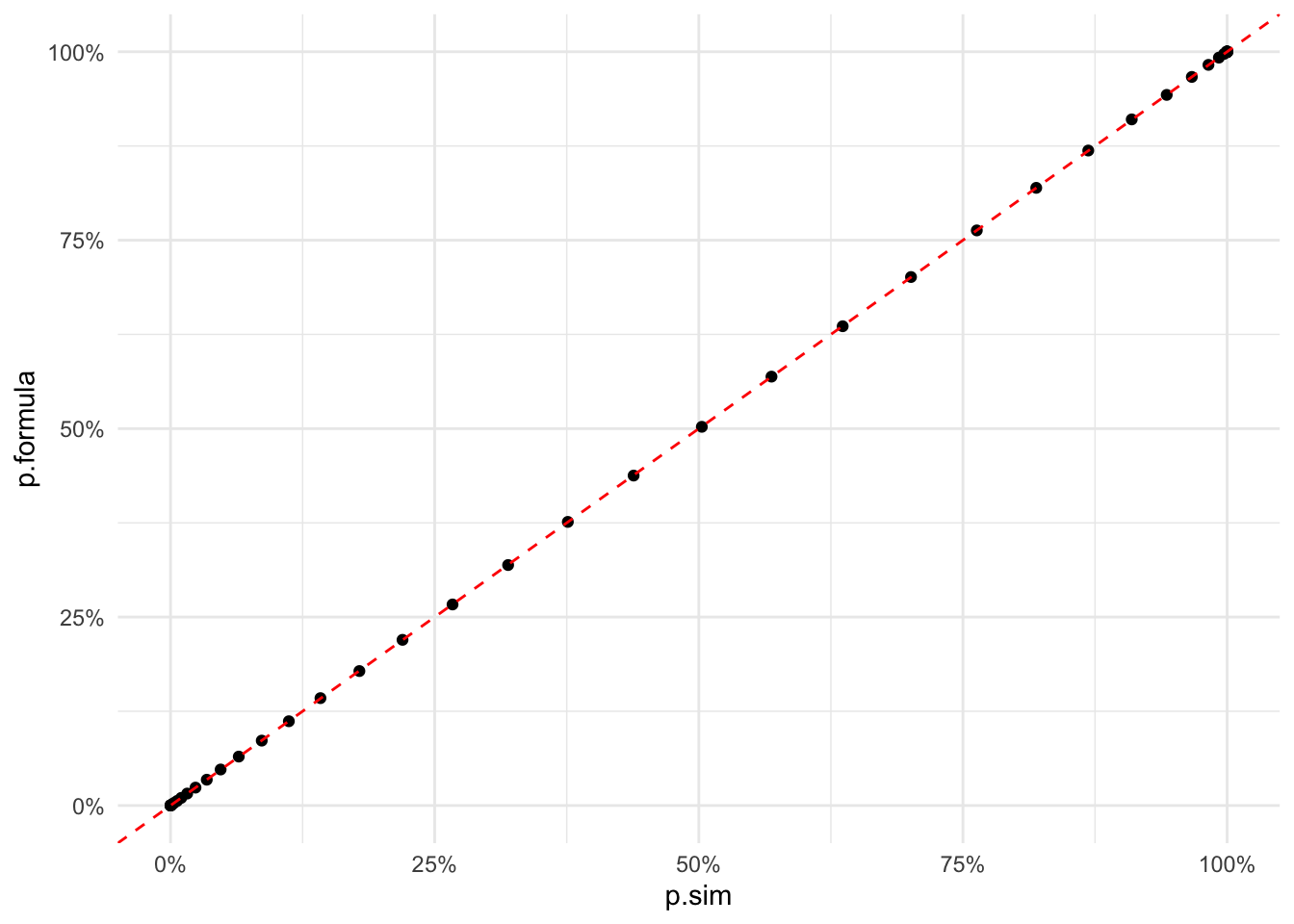

The results match the simulation very well. Hooray!

Yet another generalization

I was staring at the third case solution and realized that the terms can be simplified.

The second term $\frac{\binom{13}{2} \cdot \binom{44}{n-8} - \binom{13}{1} \cdot \binom{12}{1} \cdot \binom{44}{n-8}}{\binom{52}{n}}$ can be simplified as

\[ \begin{aligned} \frac{\binom{13}{2} \cdot \binom{44}{n-8} - \binom{13}{1} \cdot \binom{12}{1} \cdot \binom{44}{n-8}}{\binom{52}{n}} &= \frac{\binom{44}{n-8}}{\binom{52}{n}} \cdot [\binom{13}{2} - \binom{13}{1} \cdot \binom{12}{1}]\\ &= \frac{\binom{44}{n-8}}{\binom{52}{n}} \cdot [\frac{13 \cdot 12}{2} - (13 \cdot 12)]\\ &= \frac{\binom{44}{n-8}}{\binom{52}{n}} \cdot (-\frac{13 \cdot 12}{2})\\ &= -\frac{\binom{44}{n-8}}{\binom{52}{n}} \cdot \binom{13}{2} \end{aligned} \]

I have a hunch that although the third term $\frac{\binom{13}{3} \cdot \binom{40}{n-12} - \binom{13}{2} \cdot \binom{11}{1} \cdot \binom{40}{n-12} + \binom{13}{1} \cdot \binom{12}{2} \cdot \binom{40}{n-12}}{\binom{52}{n}}$ looks scary, it can also be simplified.

\[ \begin{aligned} \frac{\binom{13}{3} \cdot \binom{40}{n-12} - \binom{13}{2} \cdot \binom{11}{1} \cdot \binom{40}{n-12} + \binom{13}{1} \cdot \binom{12}{2} \cdot \binom{40}{n-12}}{\binom{52}{n}} &= \frac{\binom{40}{n-12}}{\binom{52}{n}} \cdot [\binom{13}{3} - \binom{13}{2} \cdot \binom{11}{1} + \binom{13}{1} \cdot \binom{12}{2}]\\ &= \frac{\binom{40}{n-12}}{\binom{52}{n}} \cdot \binom{13}{3} \end{aligned} \]

because

\[ \binom{13}{2} \cdot \binom{11}{1} - \binom{13}{1} \cdot \binom{12}{2} = \frac{13!}{11! \cdot 2!} \cdot \frac{11!}{10!} - \frac{13!}{12!} \cdot \frac{12!}{10! \cdot 2!} = 0 \] This means that the formula can be dramatically simplified to

The alternating signs of the second and third terms immediately reminded me of the inclusion-exclusion principle technique in combinatorics. I wonder if the general formula can be as simple as the following.

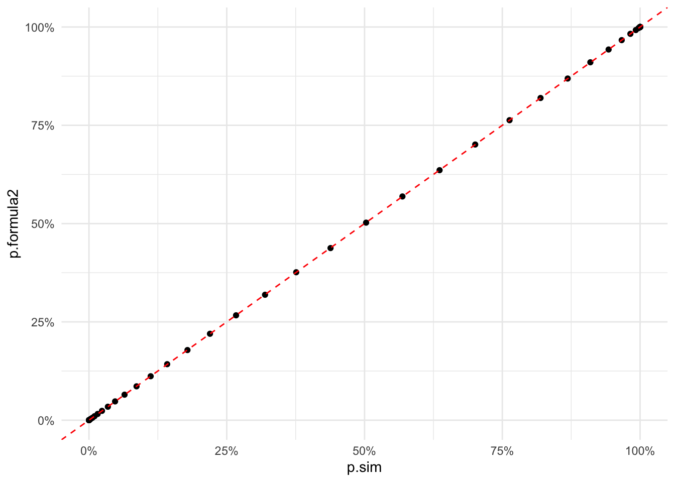
\[ P(k \geq 1, n) = \sum\limits_{K=1}^{13} (-1)^{K+1} \cdot \frac{\binom{13}{K} \cdot \binom{52-4K}{n-4K}}{\binom{52}{n}} \]

prob3 <- function(n) {
  sum(
    map_dbl(
      1:13,
      ~(-1)^(.x+1) * choose(13, .x) * choose(52-4*.x, n-4*.x) / choose(52, n)
    )
  )
}
tibble(
  n = 0:52,
  p = map_dbl(n, prob3)
) %>%
  ggplot(aes(x = n, y = p)) +
    geom_point()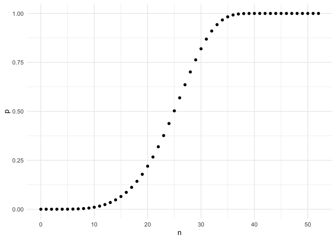

I plot the results against the simulation results and they match perfectly.

df.sim %>%
  rename(p.sim = p) %>%
  mutate(p.formula2 = map_dbl(n, prob3)) %>%
  ggplot(aes(x = p.sim, y = p.formula2)) +
    geom_point() +
    geom_abline(aes(intercept = 0, slope = 1), color = "red", linetype = "dashed") +
    scale_x_continuous(label = percent) +
    scale_y_continuous(label = percent)

Streeling

The journey of discovering four-of-a-kind in a standard deck of cards